The third camp of Auschwitz does not exist in the museum. It is a village with houses and gardens, and next to it a chemical plant that has never ceased operating since IG Farben built it with slave labor, mainly Jews. The war ended, the owner changed, the factory kept running. Every morning people clock in there.
No one guards this area. No one stands in line to see it. Eighty years of weather have been working on the brick.
Light only moves forward. I do too. That is exactly what carrying light looks like.
This is not AI art. No generative model painted, styled, or hallucinated anything into this scene. A spectral reconstruction model expands a single linear raw capture into a dense spectral cube spanning the visible and near-infrared. From that cube, a Spectral Angle Mapper (SAM) compares every pixel against a library of known spectra.
Here is exactly what the spectral angle computes:
For every pixel in the scene, we take its reconstructed spectrum \( \mathbf{s} \) (its reflectance across many narrow wavelength bands). We compare that pixel spectrum against a library of known reference material spectra \( \mathbf{r} \). The spectral angle \( \theta \) is the angular distance between these two vectors in \( n \)-dimensional band-space:
I was first introduced to Einstein’s special theory of relativity by a math teacher whose husband, a mathematician, had worked on Einstein’s field equations. Around that time Roger Penrose visited my university and I listened to his lecture. Penrose, together with Hawking, had shown that general relativity predicts the conditions of its own breakdown. That is the theory at its most extreme. The same theory at its least dramatic says something about an airplane. Fly to Tokyo and you land a few nanoseconds displaced from everyone who stayed home. It is real and it has been measured, though not as a clean demonstration of velocity alone. For an airliner, the velocity term that slows the clock competes with the altitude term that speeds it up, and in 1971 Hafele and Keating flew cesium clocks east and west around the world and recorded offsets of opposite sign for the two directions.1
After graduating college, I worked with some folks who had just finished a project on the super collider in Waxahachie and another group out of France and Geneva. It was then that I first started to think about time as something a particle carries with it. Certain particles are created high in the atmosphere and should fall apart long before they ever reach the ground. They arrive anyway. They arrive because they are moving fast enough that their own clock runs slow compared to ours, which buys them the trip down. Rossi and Hall measured this in 1941,2 and particle accelerators have confirmed it since to very high precision. Nothing about the particle itself changes. What changes is the relationship between its clock and ours.
Now the train. Einstein asked us to imagine a long, straight railway track with a train moving along it at a steady speed. Lightning strikes twice: once at the front of the train and once at the rear. On the ground, an observer stands exactly halfway between the two points where the lightning hit. She sees the light from both flashes arrive at the same moment, so she concludes the flashes were simultaneous.
On the train, a passenger sits exactly in the middle of the car. In the ground observer’s frame, the forward flash reaches the passenger first because the train carries her toward the oncoming forward light and away from the rear light. But the passenger herself is at rest in her own inertial frame; for her, light travels at speed c from both ends, and the distances to the front and rear of the car are identical. Since the forward flash arrives before the rear flash despite equal distances and equal light speed, it must have been emitted first in her frame. The two strikes are simultaneous for the ground observer, yet sequential for the passenger.
So did the strikes occur at the same time or not? In special relativity, the question has no absolute answer. The two events are spacelike-separated; no signal could travel from one strike to the other, so their temporal order is frame-dependent. Both observers are correct within their respective frames. There is no universal “now,” and simultaneity depends entirely on your state of motion.
This relativity of time becomes vivid with a light clock. Imagine a spaceship carrying a photon bouncing vertically between two mirrors. To someone on board, each round-trip is a simple up-and-down tick. To an observer on the ground, the photon traces a longer diagonal path because the mirrors move between bounces. Since the speed of light is the same for all observers, the diagonal journey takes longer. So the moving clock is seen to run slow. This is time dilation.
A word about the spaceship, because it is the part people stop on. There is nothing exotic about it. Time only stretches by an amount worth noticing when something travels at a good fraction of the speed of light, and nothing you can ride travels remotely that fast. A train is far too slow. An airplane is too slow, which is why the effect on one is measured in billionths of a second. So the thought experiment needs a vehicle that could actually reach those speeds, and a spaceship is simply the most convenient one to picture, because space is the only place with room enough to get up to speed and nothing in the way. Einstein used trains because a train was the fast thing of his day. The vehicle is a stand-in for speed and nothing else. The point is never the ship. The point is what happens to the clock inside it.
Time dilation is not a metaphor. A traveler moving at high speed ages less than those who stay behind. If you board a spaceship and accelerate to a significant fraction of light speed, you can travel years on your own clock while centuries pass on Earth. This is forward time travel, allowed by special relativity. Backward time travel, however, is not. General relativity offers theoretical loopholes: Gödel’s rotating universe,3 wormholes,4 the interior of a spinning black hole. Each fails for its own reason. Wormholes need exotic matter with negative energy density. Gödel’s solution describes a universe that rotates, which ours does not appear to do. The closed paths inside a spinning black hole sit behind a horizon nothing returns through. Hawking’s chronology protection conjecture suggests the universe forbids closed timelike curves outright.5 Practically, you can journey into the future, but you can never send a message to the past.
That irreversibility is the heart of the matter. The past is sealed. We can only move forward, carrying what we have learned.
What clung to me, what I still carry in my bones, is the cruel elegance of the instrument itself. Those trains, those spaceships: they aren’t just physics. They are lenses. Tools for seeing exactly what light permits and what it ruthlessly forbids.
And thirty years after that miracle year of 1905, Einstein aimed that same sharp, unforgiving lens away from the stars and straight into the quantum mess. He was looking for a new foothold, a new way of seeing the chaos underneath.
In 1935, Albert Einstein and his colleagues Boris Podolsky and Nathan Rosen published a seminal paper arguing that the quantum-mechanical description of physical reality is incomplete.6 The claim was not that quantum mechanics predicts wrongly. It was that a theory can predict correctly and still fail to describe everything that is there. They built the argument on a pair of particles prepared so that measuring the position or the momentum of one lets you predict the corresponding quantity for the other, at any separation, without disturbing it.
Two attributions are worth getting right, because the popular account collapses them. The familiar spin version of the argument (two-outcome measurements along chosen axes, the form in which nearly every modern discussion is conducted) is Bohm's reformulation from 1951, not the 1935 paper.7 And the word entanglement is not Einstein's either; Schrödinger introduced it later that same year, writing in reply.8
It is the quintessential example of a problem in which the whole contains information that cannot be inferred from looking at one part in isolation. An entangled pair can be prepared in a joint quantum state in which particular measurements produce strongly correlated results. Conservation laws can impose those relationships; total angular momentum has to add up. The result is not that each particle secretly carries a classical answer waiting to be revealed, but that quantum mechanics assigns probabilities and correlations to the joint system.
And the correlation is not created by the act of measurement. It is fixed at preparation, written into the joint state rather than into either particle on its own, which is a different claim from saying each particle quietly carried its own answer all along. Bell's result below rules that second reading out. Measuring one particle reveals it, and updates what you should expect from a measurement on the partner, regardless of the distance separating them. That distinction is the whole ballgame, because it is precisely why entanglement cannot be used as a telephone. The formal statement is the no-communication theorem: no local operation on one half of an entangled pair changes the measurement statistics available at the other half. The marginal distribution at each end is untouched, whatever is done at the far end. You need the classical record from both ends, brought together at light speed or slower, before the correlation becomes visible at all. The strangest object in physics still cannot carry a single word backward, or even sideways, faster than light.
So the strange thing about entanglement is not that it provides a faster-than-light telephone; it is that nature permits correlations between separated measurements that cannot be reproduced by ordinary local hidden-variable theories. Einstein objected to the implications of that picture. Bell showed in 1964 that the objection was testable,9 and experiment has since answered. Aspect, Dalibard, and Roger's 1982 measurement with time-varying analyzers10 left two gaps open, the locality loophole and the detection loophole, and both were closed in 2015 by a set of experiments that violated Bell inequalities with no significant loophole remaining.11,12,13 The 2022 Nobel Prize in Physics recognized this line of work. Local hidden variables are gone. Einstein was wrong about the conclusion and right that the question was worth forty years of somebody's life.
The EPR Analogy, and Where It Stops
While the EPR debate centered on the foundations of quantum mechanics, its deeper philosophical lesson, that direct observation can miss profound relationships within a system, resonates with modern imaging. In each case, information that is not apparent from an isolated measurement becomes accessible when measurements are considered together and interpreted through an appropriate mathematical model.
Just as the naked eye perceives only a fraction of the electromagnetic spectrum, a standard RGB sensor records only three broad spectral responses. The information discarded between and beyond those responses can contain clues about the chemical and physical properties of a material. Multispectral and hyperspectral imaging address this limitation by measuring, or in some cases estimating, how materials interact with light across a broader spectral range, and mathematical reconstruction can then infer spectral structure that is not directly represented in the original RGB observation.
The analogy is not that spectral correlations are quantum entanglement. They are not, and the difference in depth is enormous. It is only that both problems reveal the same limitation in taking a partial observation as the whole story.
Silicon Photonic Architecture The realization of this physics in modern hardware is constrained by the physical dimensions and properties of the semiconductor used to capture it. The interaction of incident photons with the silicon lattice, generating electron-hole pairs, is the primary physical process underlying photon detection in a conventional silicon image sensor, and that process sets hard boundaries at both ends of the range.
Silicon's indirect bandgap is approximately 1.1 eV, so photodiode response falls away as wavelengths approach roughly 1100 nm and there is no photoelectric detection beyond it. At the other end, absorption depth collapses: on the order of a few nanometres in the ultraviolet against hundreds of microns in the near-infrared. Ultraviolet photons are absorbed before they can reach the depth at which a front-illuminated sensor's photodiodes sit, which is the substantive reason back-illumination matters for short-wavelength work rather than a marketing distinction.
The Spectral Gatekeeper Before any of that, almost every camera bonds a UV/IR-cut filter directly into the stack above the sensor. That filter, not the lens glass, is the dominant constraint on accessible spectral range: it typically passes roughly 400–650 nm and rejects wavelengths to either side by orders of magnitude. No amount of downstream processing recovers a band the filter rejected, so any work outside that window is a question of optics and filtration rather than algorithms.
A second consequence is easy to miss. Bayer color-filter dyes leak in the near-infrared; past roughly 800 nm all three channels become nearly transparent and nearly identical. Beyond the visible window a silicon sensor therefore stops behaving as a trichromatic device and behaves more like a monochrome detector carrying three largely redundant channels, which means wavelength discrimination in that region cannot come from the color filter array at all.
Sensor Architecture The core of this pipeline is a modern back-illuminated CMOS sensor, optimized for high-resolution imaging and radiometric capture.
Active Sensing Area: The sensor's physical dimensions matter because they influence the total photon flux the device can collect for a given scene and exposure, and therefore the achievable Signal-to-Noise Ratio. No downstream algorithm can recover photons that were never recorded.
Pixel Pitch: Native photodiode pitch varies widely by format, from around a micron in small-format sensors to several microns in full-frame. Pitch, however, is usually not the binding limit.
Diffraction, Not Sampling At realistic working apertures the optics run out of resolution before the pixel grid does. The Airy disc radius is approximately 1.22λN; at f/8 and 550 nm that is about 5.4 µm, several times the pitch of a small-format sensor and larger than a typical full-frame photosite. Stopping down to gain depth of field across a textured surface therefore buys resolution loss at a predictable rate. Fine fiber structure in a document is recoverable only when aperture, wavelength, and working distance are chosen such that the optical transfer function still passes those spatial frequencies. Adding pixels does not help once diffraction has already removed the detail.
Mode Selection The choice between binned and unbinned modes depends on the analysis requirements, and the SNR arithmetic depends on where the binning happens and which noise source dominates.
True charge-domain binning—combining photocharge from neighboring photodiodes before the sense node and before readout—keeps the read-noise contribution essentially constant while the signal scales with the number of pixels summed. In the read-noise-limited regime a 2×2 operation can therefore improve SNR by up to a factor of four. Many modern CMOS sensors, however, implement only digital summation after independent digitization of each pixel, or a hybrid scheme in which charge sharing is possible in one direction only. In the pure digital case the signal still multiplies by four while uncorrelated read noise grows by the square root of four, a factor of two, limiting the SNR gain to a factor of two. In the shot-noise-limited regime (bright scenes, long exposures, controlled illumination) neither approach exceeds a factor of two, because shot noise itself scales as the square root of the collected signal. Binning remains a low-light tool; whether the spatial cost is worthwhile is decided by which noise term actually dominates the exposure.
Full-resolution (native sampling) mode is preferred when spatial detail is the priority—resolving fine fiber patterns in historical documents or detecting micro-scale material boundaries—subject to the diffraction limit above.
The Optical Path The light reaching the sensor passes through a multi-element lens assembly with a fast maximum aperture. A spectral imaging system measures a combination of the material's spectral reflectance R(λ), the illumination spectrum, the optical transmission T(λ), the detector response, and other system characteristics. Modern optical glass and coatings attenuate particular wavelengths, especially toward the near-UV, so those effects must be characterized during calibration if measurements are intended to be quantitatively meaningful. Some coated modern lenses cut off the near-UV so sharply that older uncoated or quartz-element designs are the practical choice for that end of the range.
Calibration: The Three Frames You Cannot Skip A spectral measurement is not a photograph, and the forward model above makes the requirement explicit. Recovering R(λ) means dividing out everything in that product chain that is not the material.
Dark frame: matched exposure time and sensor temperature with no light reaching the sensor, subtracted to remove black-level offset and dark current. Both are temperature-dependent, so the frame has to be acquired close in time and condition to the measurement rather than reused from an earlier session.
Flat field: uniform illumination of a spectrally neutral surface, divided out to remove lens vignetting, pixel response non-uniformity, and illumination falloff across the field. All three are wavelength-dependent, so a single flat does not serve every band.
White reference: a diffuse reflectance standard of known spectral reflectance, imaged under the same illumination in the same geometry. This is what converts raw signal into reflectance rather than an arbitrary sensor unit. Without it the pipeline produces numbers that are internally consistent and externally meaningless. Reflectance is a ratio, and something has to be the denominator.
The Digital Container: DNG and Linearity The accuracy of computational imaging depends heavily on the integrity and characterization of the input data. The Adobe DNG specification can provide a standardized container for raw or rendered image data, but the presence of a DNG extension by itself does not guarantee scientific linearity or calibrated radiometric measurements. The actual camera data, conversion path, metadata, and calibration procedure all matter.
Scene-Referred Linearity For spectral reconstruction, the important property is preservation of a useful linear relationship between recorded sensor signal and scene radiance over the relevant operating range. Raw sensor measurements can generally be treated as approximately linear with respect to accumulated signal before nonlinear display transformations are applied, but black-level offsets, gain, saturation, noise, color-filter responses, and other camera-specific characteristics must be accounted for. Linear image data is not synonymous with photon counts; it is calibrated or calibratable sensor signal.
Gain Maps and Aesthetic Metadata Modern raw-image ecosystems can carry metadata describing transformations, calibration information, or image-rendering behavior separately from the underlying image data. This separation is valuable for scientific workflows because the computational pipeline can choose which transformations are appropriate for measurement and which belong only to visual presentation.
Scientific Stewardship: By keeping measurement-oriented data separate from aesthetic rendering decisions wherever possible, the pipeline avoids allowing display-oriented processing to be confused with the underlying signal used for spectral analysis. The goal is not simply an attractive image; it is a reproducible, characterized measurement from which computational inference can be performed.
Algorithmic Inversion: From 3 Channels to a Dense Spectral Grid Recovering a high-dimensional spectral curve S(λ), potentially comprising hundreds of narrow bands sampled at nanometre-scale intervals, from a low-dimensional RGB input is an ill-posed inverse problem. It is worth being precise about why, because "ill-posed" undersells the situation.
The camera's three spectral sensitivity functions span a three-dimensional subspace of a function space with hundreds of dimensions. Any spectrum lying in the null space of that projection, the metameric blacks, produces identically zero response in all three channels. Not approximately zero: zero. Two spectra differing by a metameric black are the same RGB triple, and no algorithm recovers what the null space swallowed. Reconstruction works instead by ruling out the physically implausible members of that infinite family, using calibration data, physical constraints, statistical priors, and, in learned systems, the distribution represented in the training data. The information loss is a theorem about the projection, not a caveat about implementation quality: no amount of engineering recovers what the null space swallowed. What engineering does determine is how good the remaining guess is, and that depends on how closely the real material resembles what the model was shown.
Wiener Estimation (The Classical Baseline) The classical approach is linear minimum mean-square-error estimation, minimizing expected squared error between estimated and actual spectra through a matrix estimator:
\(W = K_r M^T (M K_r M^T + K_n)^{-1}\)
Here M is the system matrix combining illumination, optical transmission, filter response, and detector sensitivity; Kr is the covariance matrix of the spectral reflectances expected in the sample population; and Kn is the noise covariance. The estimator is optimal among all estimators only when spectra and noise are jointly Gaussian and their second-order statistics are known. Otherwise it is the best linear estimator, which is a materially weaker claim. Kr is where the assumptions hide: the result is only as good as the population you have assumed you are measuring, which is why a Wiener estimator built for one class of material degrades on another.
For decades, linear statistical estimation provided an interpretable route from a low-dimensional observation to an n-band estimate, and it remains a useful reference against which learned methods can be judged. But as a global linear operator it cannot exploit the spatial context or nonlinear relationships that help resolve some of the ambiguity created by spectral compression.
State-of-the-Art: Transformers and Mamba For high-end computational environments, predictive neural architectures can leverage spatial and spectral correlations to resolve ambiguities that simple global linear models cannot. None of them escape the null-space argument above; what they improve is the quality of the prior, not the information content of the measurement. That prior is only as reliable as the distribution on which it was trained. Spectra, illuminants, or material classes that lie outside the training support can produce plausible-looking reconstructions whose errors are invisible to ordinary visual inspection and are not flagged by the network itself. Cross-validation against measured reference spectra under the actual illumination and geometry remains essential; without it the output is an informed guess whose confidence interval is unknown.
MST++ (Spectral Attention Architecture)14: The Multi-stage Spectral-wise Transformer represents a significant development in learned spectral reconstruction. Unlike a single global matrix estimator, MST++ uses attention mechanisms to model relationships between spectral features, allowing the network to learn nonlinear relationships that are difficult to capture with a fixed linear operator. Attention is computationally expensive, particularly as token dimensions and image resolution grow, making memory management important at high resolutions.
State Space Models (Efficient Sequence Processing)15: A newer family of architectures replaces conventional attention with state-space mechanisms. Selective state space models such as Mamba discretize a continuous state-space formulation into a form suitable for efficient sequence processing. Their computational characteristics can be favorable for long sequences, and recent research has adapted Mamba-inspired architectures to spectral reconstruction and spectral compressive imaging.16,17 These approaches are attractive for large images because they model long-range dependencies without relying exclusively on quadratic self-attention. Actual memory and computational cost depends on the architecture and implementation rather than being universally linear in every dimension of the problem.
Multi-Frame Super-Resolution: Approaching the Optical Limit The sampling limits of a single sensor frame can be partly overcome through multi-frame super-resolution compositing, where multiple precisely registered exposures containing sub-pixel shifts are combined into a higher-resolution representation.
What this recovers, precisely, is information above the sampling limit that the optics passed and the pixel grid could not record: aliased and undersampled structure. It cannot exceed the diffraction limit, because that information never arrived at the sensor plane in the first place. The final result remains bounded by the lens's optical transfer function, aberrations, sensor noise, subject and platform motion, registration accuracy, and the information actually present in the source exposures. The objective is not to manufacture detail from nothing, but to make better use of information distributed across multiple measurements.
For spectral work, though, the more valuable gain has nothing to do with resolution. Sub-pixel offsets place different photosites, and therefore different color-filter positions, over the same point on the subject, so the composite can carry genuinely measured R, G, and B values at each output location instead of demosaic-interpolated estimates. Demosaicing invents two of every three color values per pixel, and invents them from neighbouring pixels, which corrupts exactly the per-pixel channel ratios that spectral reconstruction consumes as its input. Eliminating that interpolation matters more to spectral fidelity than the additional pixels do.
These composites preserve the linearity and calibration characteristics of the source data when the processing pipeline is designed appropriately, allowing spectral reconstruction to operate on the resulting representation. The data footprint scales accordingly: floating-point spectral arrays become enormous, and a complete high-resolution multispectral cube may require many gigabytes of storage. The increased spatial detail can enable micro-scale textural analysis that would otherwise be lost, revealing deposition patterns, brushstroke gradients, and surface anomalies at scales approaching the practical resolving capability of the optical system.
Computational Architecture Achieving multispectral precision requires a robust, modular architecture capable of handling massive arrays across a high-dimensional latent space, which in practice means a scientific Python stack running on hardware with substantial memory and bandwidth.
Ingestion: raw decoding is worth one specific warning, because it is a common and silent source of error. Raw decoders do not return linear data by default. Typical defaults apply a gamma curve and automatic brightness scaling, so obtaining sensor-oriented linear values requires disabling those explicitly and handling black-level subtraction as a separate step. Everything downstream inherits whatever was wrong here.
Processing and Analysis: high-performance array libraries handle the matrix algebra required to transform or estimate spectral representations from RGB data, with additional scientific libraries for geometric transforms, image restoration, and spatial filtering, and a plotting layer for spectral signature graphs and false-color composites.
Data Footprint: the scale is significant. A single high-resolution frame converted to floating-point precision produces large files. Intermediate files can exceed hundreds of megabytes for a single three-channel layer, while a full n-band multispectral cube scales proportionally with band count and spatial dimensions. Super-resolution composites multiply those requirements further, producing intermediate arrays that can exceed many gigabytes and necessitating careful memory management, fast storage, and substantial memory bandwidth.
The Spectral Solution Two blue pigments make the argument concrete. Ultramarine and azurite are difficult to separate reliably by eye or by RGB response, and trivially separable once the near-infrared is available, for reasons that come directly from their chemistry:
Spectral Feature
Ultramarine (Lapis Lazuli)
Azurite (Copper Carbonate)
Origin of colour
The S3− radical anion held in the sodalite-type lazurite lattice, producing broad absorption centred near 600 nm
Cu2+ d-d electronic transitions in a basic copper carbonate
Visible-region behaviour
Strong reflectance in the blue-violet region; reduced reflectance through the orange-red where the 600 nm absorption sits
Blue reflectance with a greener bias than ultramarine; spectral shape influenced by particle size, concentration, and binder
Near-infrared behaviour (the discriminator)
Highly reflective through the NIR; remains bright in infrared reflectography
The same Cu2+ transitions produce strong broad absorption extending through the NIR; goes dark in infrared reflectography
Practical requirement
The NIR separation lies outside the roughly 400–650 nm window a stock camera passes, so it depends entirely on the optical and filtration choices discussed above. Inside the visible window alone the two pigments can be genuinely ambiguous.
Note: Measured values vary with pigment composition, particle size, binding medium, concentration, substrate, aging, illumination, and instrument calibration. The NIR contrast between these two is robust because it follows from electronic structure rather than from preparation, but quantitative identification still requires comparison against reference spectra acquired under controlled conditions.
Completing the Picture The successful analysis of complex material properties relies on a convergence of rigorous physics and advanced computation.
Photonic Foundation: A modern back-illuminated CMOS sensor provides high-SNR photonic capture across silicon's usable range, with readout mode driven by which noise regime the exposure actually sits in.
Spectral Access: The accessible range is set by the UV/IR-cut filter first, silicon's 1.1 eV bandgap second, and the optics third. Extending past the visible window is a hardware question, not a software one.
Sensor Diversity: An ingestion layer can normalize black level, white balance, and color filter array geometry across proprietary and standard raw formats. What that produces is format consistency, not radiometric equivalence. Two bodies with different spectral sensitivity functions record different projections of the same spectrum, and harmonizing the containers does not harmonize the measurement. Cross-body comparability requires per-camera SSF characterization, measured against a monochromator or estimated from a calibrated target set, and until a body has been characterized its reconstructions are internally usable but only loosely comparable to another body's.
Data Integrity: A properly characterized raw workflow or linear DNG provides a foundation for preserving scene-referred data, but the file format alone guarantees nothing about radiometric accuracy. Dark, flat, and white-reference frames remain non-optional.
Algorithmic Precision: Wiener estimation remains the classical reference point, while MST++ and Mamba-based architectures model complex nonlinear relationships between image observations and spectral structure. Their output is inference constrained by a learned prior, not recovery of information the camera never measured. Performance outside the training distribution is not guaranteed and must be checked against physical references. Multi-frame compositing improves spatial sampling and, more importantly here, removes demosaic interpolation from the spectral input.
Physical Pattern Analysis: Spectral reconstruction alone cannot resolve every ambiguity. Materials that are spectrally similar can often be separated by their spatial characteristics: texture, edge morphology, and distribution across a surface. Supplementing per-pixel spectral classification with geometric analysis of the spatial domain gives a second, independent axis of evidence, closing a gap that purely spectral methods leave open.
Historical Continuity: The EPR debate of 1935 forced physicists to confront the possibility that a complete description of a system could not be reached through classical intuition about its individual parts. Modern spectral imaging presents a different and far less profound problem that rhymes with it: materials carry structured information across wavelength that is invisible to trichromatic vision. In both cases, completeness requires looking beyond what a single direct observation provides.
Hardware, calibration, file-format stewardship, and reconstruction converge on one thing: a spectral witness to what ordinary vision alone cannot tell us.
And what about the paint? Here is a physical sample: pigment, substrate, history compressed into matter. Light passes through it, scatters from it, carries fragments of its story: yet the full truth remains hidden until we choose to look deeper. Every layer, every faded stroke, every chemical trace is a silent archive. We are not just observers; we are custodians of that archive. When we build tools to see beyond the visible, we are not merely extending sight: we are accepting a quiet responsibility: to bear witness honestly, to preserve what time would erase, to honor what has been made and endured.
Light can expose structure. It cannot carry history.
That part is on us.
We can choose to let the machines we build serve memory rather than erasure, dignity rather than classification, truth rather than convenience. The past does not ask for perfection: it asks only that we refuse to let it be forgotten. In every reconstruction, in every layer we uncover, we have the chance to listen again to what was silenced. That is not just engineering. That is the work of being human.
But tonight, sitting here in the dark, I realize I am still riding that same damn train. Hurtling toward one flash, watching the other recede into a past I can never touch, never text, never warn. Information can race forward, people can race forward, but nothing, nothing gets to go back. We are all just riders, carried away from every moment we have already survived, looking for answers in the one direction the universe actually lets us move. Forward. Always forward. And that is the most beautiful, devastating thing I know.
References
1 Hafele, J. C., & Keating, R. E. (1972). Around-the-World Atomic Clocks: Predicted Relativistic Time Gains; Observed Relativistic Time Gains. Science, 177(4044), 166–168; 168–170.
2 Rossi, B., & Hall, D. B. (1941). Variation of the Rate of Decay of Mesotrons with Momentum. Physical Review, 59(3), 223–228.
3 Gödel, K. (1949). An Example of a New Type of Cosmological Solution of Einstein's Field Equations of Gravitation. Reviews of Modern Physics, 21(3), 447–450.
4 Morris, M. S., & Thorne, K. S. (1988). Wormholes in spacetime and their use for interstellar travel: A tool for teaching general relativity. American Journal of Physics, 56(5), 395–412.
5 Hawking, S. W. (1992). Chronology protection conjecture. Physical Review D, 46(2), 603–611.
6 Einstein, A., Podolsky, B., & Rosen, N. (1935). Can Quantum-Mechanical Description of Physical Reality Be Considered Complete? Physical Review, 47(10), 777–780.
7 Bohm, D. (1951). Quantum Theory. Prentice-Hall. (Spin reformulation of the EPR argument.)
8 Schrödinger, E. (1935). Discussion of Probability Relations between Separated Systems. Proceedings of the Cambridge Philosophical Society, 31(4), 555–563.
9 Bell, J. S. (1964). On the Einstein Podolsky Rosen paradox. Physics Physique Физика, 1(3), 195–200.
10 Aspect, A., Dalibard, J., & Roger, G. (1982). Experimental Test of Bell's Inequalities Using Time-Varying Analyzers. Physical Review Letters, 49(25), 1804–1807.
11 Hensen, B., et al. (2015). Loophole-free Bell inequality violation using electron spins separated by 1.3 kilometres. Nature, 526, 682–686.
12 Giustina, M., et al. (2015). Significant-Loophole-Free Test of Bell's Theorem with Entangled Photons. Physical Review Letters, 115, 250401.
13 Shalm, L. K., et al. (2015). Strong Loophole-Free Test of Local Realism. Physical Review Letters, 115, 250402.
14 Cai, Y., Lin, J., Lin, Z., Wang, H., Zhang, Y., Pfister, H., Timofte, R., & Van Gool, L. (2022). MST++: Multi-stage Spectral-wise Transformer for Efficient Spectral Reconstruction. Proceedings of the IEEE/CVF Conference on Computer Vision and Pattern Recognition Workshops (CVPRW).
15 Gu, A., & Dao, T. (2023). Mamba: Linear-Time Sequence Modeling with Selective State Spaces. arXiv:2312.00752.
16 Zhang, Y., Li, L., Lin, Q., Ming, Z., Yu, F., & Leung, V. C. M. M3SR: Multi-Scale Multi-Perceptual Mamba for Efficient Spectral Reconstruction. [venue and year to be completed]
17 Qin, M., Feng, Y., Wu, Z., Zhang, Y., & Yuan, X. Detail Matters: Mamba-Inspired Joint Unfolding Network for Snapshot Spectral Compressive Imaging. [venue and year to be completed]
Provenance · Integrity Record
Canonical file hashes · SHA‑512
Hashes are of the byte-identical JPEGs converted from raw sensor data. Verify with sha512sum -c SHA512SUMS.
I looked up and saw him, suddenly free from above me, floating in open air. He’d been hovering over a pale desert portrait that looks like it has no eyes left to cry with. I didn’t wonder where he came from; he just arrived. His horn doesn’t play tunes so much as make a quiet sound that demands attention. It feels exactly like the things we keep inside, trying not to let them out, until one day the walls simply can’t hold them anymore. He isn’t quite heavenly or ghostly, just something true, finally letting go.
Provenance · Integrity Record
Canonical file hashes · SHA‑512
Hashes are of the byte-identical PNGs converted from raw sensor data. Verify with sha512sum -c SHA512SUMS.
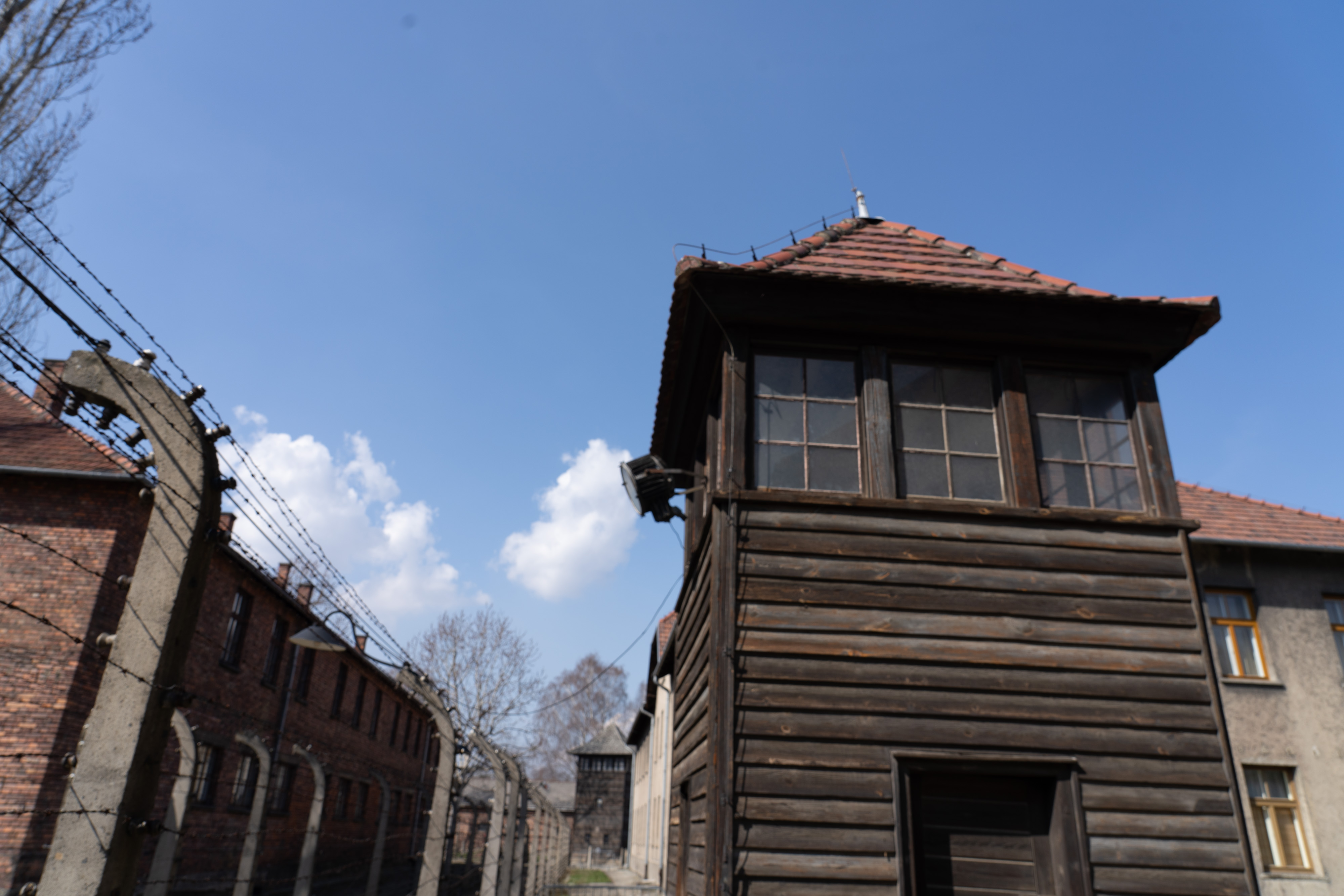
She arrived under a tower like this one, three kilometres away at Birkenau. She left as Reg. A 105, folio 9.
Auschwitz I was surrounded by a double barbed-wire fence punctuated by guard towers at regular intervals. The towers stood on the outer perimeter; the fence was electrified at high voltage. Along the fence, on the camp side, ran a gravelled strip, the "neutral zone". Camp regulations, corroborated by survivor testimony, held that guards in the towers could shoot any prisoner who entered that strip without warning. Their function was custody: to ensure that the people inside could not leave until the state had decided how they would.
flyio
On 3 September 1944, the last transport from the Westerbork transit camp to Auschwitz departed the Netherlands. It arrived at the new ramp inside Auschwitz II–Birkenau on the night of 5–6 September, after two and a half days in locked cattle wagons. Of the 1,019 Jews on the manifest, four were Franks. They appeared in sequence: Margot at 306, Otto at 307, Edith at 308, Annelies Marie at 309. By the Anne Frank House's reconstruction from the transport list and the camp number series, 648 people from the transport were registered into the camp administration after selection; 371 were sent directly to the gas chambers. The women remained at Auschwitz II–Birkenau. The men were taken to Auschwitz I, about three kilometres away; the distance and the camp's known procedures suggest they made the journey on foot. On 30 October, Margot and Anne were selected for transfer to Bergen-Belsen; the transport departed the night of 1 November and arrived on 3 November. The dates are reconstructed from survivors' letters and interviews; no transport list naming the sisters survives. Edith was left behind at Auschwitz II–Birkenau. According to the account of Rosa de Winter‑Levy, she died there in the infirmary on 6 January 1945; neither the place nor the date is confirmed by any camp record.
The Westerbork camp kept its own register. Her entry is on page 40. The pink card below is an extract citing it, preserved in her death file; the oldest documents in that file date from April 1951, so the card was most likely made in the course of postwar processing rather than at the camp. Transport: 3-9-44. Naam: FRANK. Voornamen: Annelies, M. Geboren: 12-6-29. Adres: Merwedeplein 37, Asd. It is among the last documents in the state's custody of her to record the street where she lived.
Westerborkregister · Frank, Annelies M. · transport 3-9-44 Nationaal Archief, Den Haag · 2.09.34.02, inv.nr. 539 · public domain
Bergen-Belsen maintained a prisoner registration system, so Margot and Anne would have been registered upon arrival and assigned new numbers, as was standard practice. But shortly before British forces liberated the camp on 15 April 1945, the SS burned the prisoner registration records. The numbers Anne and Margot were assigned at Bergen-Belsen are not known; neither are their Auschwitz numbers. The women of their transport were tattooed in a numbered series, but no surviving record ties either sister to a number within it. After the Westerbork transport list of 3 September 1944, no surviving document names them at all. According to eyewitness accounts and the postwar historical consensus, they died at Bergen-Belsen of typhus, probably in February 1945. The dating rests on those witness statements, on the 7 February 1945 transport list to Raguhn (which fixes the departure of witnesses who had seen them ill), on the receipt of a Red Cross parcel in late January 1945, and on the ordinary course of the disease.
For six years, the paperwork caught up slowly. The two oldest documents in her death file are forms dated 6 April 1951, in which the Commissie tot het doen van aangifte van overlijden van vermisten, the Committee for the Reporting of the Decease of Missing Persons (created under the law of 2 June 1949), wrote to the Dutch Red Cross and to the Amsterdam civil registrar to ask what was known. The Red Cross filed the Committee's request against its own record: "dossier N.R.K. 117266. Cf. concl. RK † 31 Maart 1945 te Bergen Belsen / Dld." Conclusion: died no later than 31 March 1945 at Bergen-Belsen. The Amsterdam civil registrar confirmed that no death certificate had been issued. Six years after Anne Frank's death, the municipal record said only that she had vanished and had never been declared dead.
On 7 May 1954, Johannes Kleiman, Otto Frank's colleague and one of the helpers who had hidden the Franks, wrote to the Committee as Otto's authorized representative, asking that the declarations for Margot and Anne be processed; Otto needed them to have a certificate of inheritance drawn up. The Committee acknowledged receipt on 4 June. The declaration itself was issued on 29 July 1954, in The Hague. It is the document reproduced below.
Aangifte van overlijden · No. 107658 · 's-Gravenhage, 29 Juli 1954 Commissie tot het doen van aangifte van overlijden van vermisten · Nationaal Archief 2.09.34.02, inv.nr. 539
The declaration is a typed form on light paper, numbered No. 107,658. Stamped at the top: AFSCHRIFT — copy. The printed Dutch is dense with legal procedure: Krachtens art. 2 van de Wet van 2 Juni 1949 (Stbl. No. J 227) doe ik U hierbij aangifte van het overlijden van de hieronder vermelde vermiste. By virtue of article 2 of the Law of 2 June 1949, I hereby declare the death of the missing person named below. The filled-in carbon strikes are faint: Op een en dertig Maart negentienhonderd vijf en veertig is in Bergen-Belsen in Duitsland overleden: Frank, Annelies Marie. The date is written in longhand Dutch, een en dertig Maart, the certainty the facts didn't support, spelled out word by word.
The form was sent to the Amsterdam civil registrar. Three months later, on 29 October 1954, the registrar entered the death in the municipal register in faint purple hand at the lower right: Reg. A/105. Fol. 9. Initialled and filed.
Archiefkaart · Frank, Annelies Marie Cites overlijdensakte · Burgerlijke Stand Amsterdam · Reg. A 105, Fol. 9 · d.d. 29-10-1954
The archiefkaart is Amsterdam's internal reference card for that registry entry. Printed fields in Dutch: Naam, Voornamen, Geboren op, Overleden op, Overlijdensakte opgemaakt, Bijzonderheden. The handwriting fills them in. Born 12 June 1929. Died 31 March 1945. Filed at Amsterdam on 29-10-54. Bijzonderheden (particulars): blank.
The working card that produced the date survives in the Dutch Red Cross Information Bureau's persoonsdossier on Anne Frank. It is pencil and ink, stamped 22 January 1952, a year after the statement of Lien (Lientje) Rebling-Brilleslijper, who had been imprisoned with Anne and Margot at Bergen-Belsen. In the clerk's hand at the bottom, boxed off from the rest, is the conclusion: Overleden te Bergen-Belsen niet eerder dan op 1.3.45 en uiterlijk 31.3.45. No earlier than 1 March, no later than 31 March.
Cartotheekkaartje · Frank, Annelies Marie · d.d. 22-1-1952 Nederlandse Rode Kruis, Informatiebureau · Nationaal Archief 2.19.288, inv.nr. 101677 · vervroegd openbaar gemaakt oktober 2023
The date 31 March 1945 is a bureaucratic default. It was the Committee's standard practice to date unknown deaths at the last day of the assumed month when a witness statement could establish the month. The witness statement was Brilleslijper's, given to the Dutch Red Cross on 22 January 1951. She said Anne and Margot died "around March 1945." She had put it differently elsewhere: to Otto Frank in November 1945 (the end of February or the beginning of March), and in a memoir written at his request in April 1951, where the end comes in February. The Committee picked March 31. No one then knew, and no one now knows, when Anne Frank actually died.
Her name also appears on a typed list. Lijst No. 1908. Every entry on the page is a Frank. She is fifth down: Annelies Marie, Frankfurt am Main, 12-6-1929, Bergen-Belsen, 31-3-1945. Six rows below her: Aron Moses Edward, Rotterdam, 7-8-1910, Polen, 31-3-1944. Place of death: Poland. The last day of March. Almost certainly the same administrative default, one year earlier. Near the top: Andries, Tiel, 4-3-1914, Omgeving van Auschwitz, 30-4-1943 (surroundings of Auschwitz, the last day of April). The list is one of many. This sheet was typed on 29 April 1959. It covers the letter A through the start of B.
Concentratiekamp · Lijst No. 1908 · Frank (A–Ba), page 14 Typed list of Dutch concentration-camp victims · d.d. 29-4-1959
Sources
Transport list: numbers 306, 307, 308, 309 (Margot, Otto, Edith, Anne Frank). Nederlandse Rode Kruis, Den Haag (war archive now held by the Nationaal Archief): Transportlijst Westerbork–Auschwitz, 3 september 1944 (inv. nr. 1066, Blatt 7). Otto Frank is listed at number 307 as "Frank Otto 12.5.89 Kaufman." Cited via the scholarly apparatus of the Anne Frank House Knowledge Base: Deportation to Auschwitz-Birkenau. This was the last transport from Westerbork to Auschwitz; larger transports left afterwards for other destinations, including transport XXIV/7 to Theresienstadt on 4 September 1944 with over 2,000 people.
Auschwitz-Birkenau: selection at the ramp, separation of men and women; arrival confirmed on the night of Tuesday 5 to Wednesday 6 September 1944. By the Anne Frank House's reconstruction from the transport list and camp number series, 648 of the 1,019 persons (399 men, 249 women) entered the camp administration and 371 were killed on arrival. Danuta Czech's Kalendarium der Ereignisse im Konzentrationslager Auschwitz-Birkenau gives the older standard figures for this transport: 470 registered (258 men, 212 women) and 549 killed. Anne Frank House Knowledge Base: Selections upon arrival at Auschwitz-Birkenau; Auschwitz I: the men in the Stammlager.
The new internal Birkenau ramp (Neue Rampe), operational from May 1944. Muzeum Auschwitz-Birkenau (Oświęcim): The unloading ramps and selections.
Auschwitz I: double barbed-wire fence, watchtowers, high-voltage electrification, and the "neutral zone" where prisoners could be shot. Wacław Długoborski, Franciszek Piper (eds.), Auschwitz 1940–1945. Central issues in the history of the camp, Oświęcim: Auschwitz-Birkenau State Museum, 2000, vol. I, and survivor testimonies. Photographs of the preserved fence system: Muzeum Auschwitz-Birkenau: Watchtowers and fence system (Former Auschwitz I site).
Otto Frank's transfer to Auschwitz I. The Anne Frank House states that the men were taken to Auschwitz I, about three kilometres away; the camp's layout and standard practice suggest they made the journey on foot. No document explicitly records the mode of travel for this group. Anne Frank House Knowledge Base: Auschwitz I: the men in the Stammlager.
Transfer of Margot and Anne to Bergen-Belsen (selected 30 October 1944; transport departed 1 November; arrived 3 November). Dates reconstructed from survivor correspondence and interviews (letters of Margot Rosenthal and Nanette Blitz to Otto Frank; Willy Lindwer, De laatste zeven maanden, 1988; synthesis in Bas von Benda-Beckmann, Na het Achterhuis, 2020); no transport list naming Anne or Margot survives. Anne Frank House Knowledge Base: Journey to Bergen-Belsen; Arrival at Bergen-Belsen.
Registration at Bergen-Belsen. Bergen-Belsen maintained a prisoner registration system; arriving prisoners were routinely registered and assigned numbers. The SS burned these records before liberation, so the specific registration of Anne and Margot is an inference from standard camp procedure, not a documented fact. Gedenkstätte Bergen-Belsen (Lower Saxony): Register of Names; The Dead of the Bergen-Belsen Concentration Camp.
Death of Anne and Margot Frank at Bergen-Belsen. No camp record documents their deaths. The place and approximate date rest on eyewitness accounts (Brilleslijper, Blitz, Van Amerongen, and others) and subsequent historical analysis. The 31 March 1945 administrative default and the February 1945 revision are discussed in Anne Frank House: Sources for the date of death of Anne and Margot Frank in Bergen-Belsen (2015): eyewitness statements, the Bergen-Belsen–Raguhn transport list of 7 February 1945 (ITS, Bad Arolsen), a Red Cross parcel receipt of c. 23 January 1945, and the clinical course of typhus. Anne Frank House Knowledge Base: Death of Anne and Margot Frank. Official date based on Lientje Brilleslijper's 22 January 1951 statement to the Nederlandse Rode Kruis (file 117266, cartotheekkaartje of the Afwikkelingsbureau Concentratiekampen); the same Anne Frank House document records her earlier statements of 11 November 1945 and 5 April 1951, and notes that Otto Frank needed the declarations for a certificate of inheritance. Official date set by the Commissie tot het doen van aangifte van overlijden van vermisten, Dutch Ministry of Justice. Underlying archival research: Raymund Schütz, Vermoedelijk op transport (Master's thesis, Archival Science, Universiteit Leiden Instituut Geschiedenis, 2010).
Edith Frank-Holländer: death at Auschwitz II–Birkenau, 6 January 1945. The place and date rest solely on the account of Rosa de Winter-Levy; no camp record confirms them. See also the Anne Frank House Knowledge Base.
Westerbork transit camp: site memorial and documentation. Herinneringscentrum Kamp Westerbork (Hooghalen): kampwesterbork.nl.
Westerborkregister: extract card for Annelies Marie Frank, transport of 3 September 1944. Pink preprinted card citing the Westerbork register (Blz. 40) and recording surname (Frank), given names (Annelies, M.), date of birth (12-6-29), home address (Merwedeplein 37, Amsterdam), and transport date (3-9-44). Preserved in Anne Frank's overlijdensdossier at the Committee; the card's own production date is not established. The oldest documents in the dossier are the Committee's forms of 6 April 1951, so the card was most likely made in the course of postwar processing rather than at the camp. Nationaal Archief, Den Haag: Ministerie van Justitie / Commissie tot het doen van aangifte van overlijden van vermisten, toegangsnummer 2.09.34.02, inv.nr. 539. Publicly accessible; no copyright restrictions ("Volledig openbaar. Er zijn geen beperkingen krachtens het auteursrecht").
Aangifte van overlijden van vermiste (declaration of death of a missing person): Annelies Marie Frank, No. 107,658. Issued in 's-Gravenhage (The Hague) on 29 July 1954 by the Commissie tot het doen van aangifte van overlijden van vermisten (Ministry of Justice), a body established under the Wet van 2 Juni 1949 (Stbl. No. J 227) to produce paper closure for Dutch residents missing from the war. Entered by the Amsterdam civil registrar on 29 October 1954 in the Register van Overlijden, Register A 105, Folio 9. Nationaal Archief, Den Haag: toegangsnummer 2.09.34.02, inv.nr. 539. Publicly accessible; no copyright restrictions. The same document is catalogued at Yad Vashem, Record Group O.41, item 5222601. The full chronology of the Committee's handling of Anne Frank's case (6 April 1951 inquiries to the Dutch Red Cross and Amsterdam civil registrar; Kleiman's 7 May 1954 letter on behalf of Otto Frank; the Committee's 4 June 1954 acknowledgment; the 29 July 1954 declaration; the 29 October 1954 Amsterdam registration) is set out in the Nationaal Archief's public exhibition page, Het overlijden van Anne Frank wordt vastgesteld.
Cartotheekkaartje: NRK Information Bureau conclusion card, stamped 22 January 1952. Handwritten index card summarising Brilleslijper's statement and establishing the administrative bracket for the date of death: Overleden te Bergen-Belsen niet eerder dan op 1.3.45 en uiterlijk 31.3.45. References NRK Information Bureau Report 6/XIV No. 102, Opsporing Joodse Personen (Search for Jewish Persons). Preserved in Anne Frank's persoonsdossier at the Dutch Red Cross Information Bureau. Nationaal Archief, Den Haag: Het Nederlandse Rode Kruis — Informatiebureau: Persoonsdossiers, toegangsnummer 2.19.288, inv.nr. 101677 (persoonsdossier Anne Frank, vervroegd openbaar gemaakt / released ahead of schedule, October 2023).
Archiefkaart: Frank, Annelies Marie. Amsterdam civil registry reference card citing the overlijdensakte at Register A 105, Folio 9, d.d. 29-10-1954. The Stadsarchief Amsterdam holds archief- and persoonskaarten under toegangsnummer 30238, and cards of deceased persons are publicly accessible online at archief.amsterdam. The archival provenance of the specific scan reproduced above is not established here.
Typed concentration-camp victim list reproduced above. Header: CONCENTRATIEKAMP — Lijst No. 1908. Column headers: Naam / Voornaam / Plaats en datum van geboorte / Plaats en datum van overlijden. Page 14 of a larger series; typed footer dated 29 April 1959, with bilingual Dutch-French labels par typ and par contr. The format is consistent with Nederlandse Rode Kruis compilations from the postwar Afwikkelingsbureau Concentratiekampen, but the archival provenance of the scan itself is not established here.
Provenance · Integrity Record
Canonical processed file hashes · SHA‑512
Hash is of the byte-identical JPEG converted from raw sensor data. Verify with sha512sum -c SHA512SUMS.
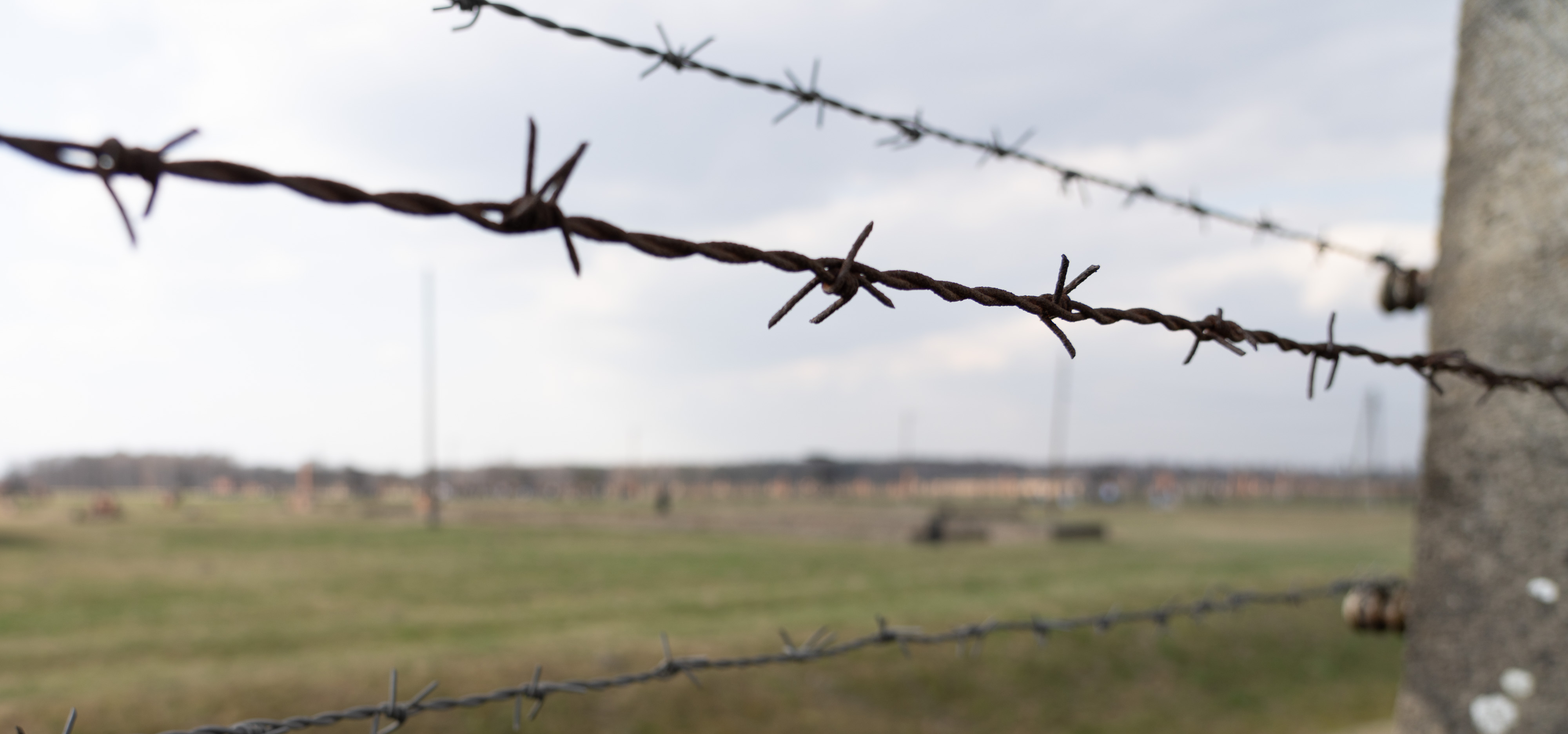
I took this photo while walking around the perimeter of Auschwitz II-Birkenau in Oświęcim, Poland. The barracks in the distance are to the left of the barracks where Edith, Margot, and Anne Frank stayed, specifically sector BIb of the women's camp.
After Birkenau, I traveled through Kraków and stopped to pick up some food and drinks for the long ride ahead, huddled up in the rail car.
Provenance · Integrity Record
Canonical processed file hashes · SHA-512
Hash is of the byte-identical JPEG converted from raw sensor data. Verify with sha512sum -c SHA512SUMS.